Statistics
Data is stochastic in nature, so an experimenter uses statistical methods on a data sample \(\textbf{x}\) to make inferences about unknown parameters \(\mathbf{\theta}\) of a probabilistic model of the data \(f\left(\textbf{x}\middle|\mathbf{\theta}\right)\). The likelihood principle describes a function of the parameters \(\mathbf{\theta}\), determined by the observed sample, that contains all the information about \(\mathbf{\theta}\) that is available from the sample. Given \(\textbf{x}\) is observed and is distributed according to a joint probability distribution function (PDF), \(f\left(\textbf{x}\middle|\mathbf{\theta}\right)\), the function of \(\mathbf{\theta}\) which is defined by
is called the likelihood function [1]. If the data \(\textbf{x}\) consists of independent and identically distributed values, then:
Classical Statistics
First we will take a look at the classical approach to statistics, so that we can then compare against the Bayesian approach. The maximum likelihood estimators (MLE) of the parameters \(\mathbf{\theta}\), denoted by \(\mathbf{\hat\theta}(\textbf{x})\), are attained by maximising \(L\left(\mathbf{\theta}\middle|\textbf{x}\right)\).
Often, not all the model parameters are of direct inferential interest however they are included as they may reduce the effect of systematic bias. These are called the nuisance parameters, \(\mathbf{\theta}_\nu\). To reduce the impact of the nuisance parameters, prior knowledge based on past measurements \(\textbf{y}\) may be included in the likelihood:
By finding the MLE for the nuisance parameters, \(\mathbf{\hat\theta}_{\nu}(\textbf{y})\), the profile likelihood can be written in terms independent of \(\mathbf{\theta}_\nu\):
The key method of inference in physics is hypothesis testing. The two complementary hypotheses in a hypothesis testing problem are called the null hypothesis and the alternative hypothesis. The goal of a hypothesis test is to decide, based on a sample of data, which of the two complementary hypotheses is preferred. The general format of the null and alternative hypothesis is \(H_0:\mathbf{\theta}\in\Theta_0\) and \(H_1:\mathbf{\theta}\in\Theta_0^c\), where \(\Theta_0\) is some subset of the parameter space and \(\Theta_0^c\) is its complement. Typically, a hypothesis test is specified in terms of a test statistic (TS) which is used to define the rejection region, which is the region in which the null hypothesis can be rejected. The Neyman-Pearson lemma [2] then states that the likelihood ratio test (LRT) statistic is the most powerful test statistic:
where \(\mathbf{\hat\theta}\) is a MLE of \(\mathbf{\theta}\) and \(\mathbf{\hat\theta}_{0}\) is a MLE of \(\theta\) obtained by doing a restricted maximisation, assuming \(\Theta_0\) is the parameter space. The effect of nuisance parameters can be included by substituting the likelihood with the profile likelihood \(L\rightarrow L_P\). The rejection region then has the form \(R\left(\mathbf{\theta}_0\right)=\{\textbf{x}:\lambda\left(\textbf{x}\right) \leq{c}\left(\alpha\right)\}\), such that \(P_{\mathbf{\theta}_0}\left(\textbf{x}\in R\left(\mathbf{\theta}_0\right)\right)\leq\alpha\), where \(\alpha\) satisfies \(0\leq{\alpha}\leq 1\) and is called the size or significance level of the test and is specified prior to the experiment. Typically in high-energy physics the level of significance where an effect is said to qualify as a discovery is at the \(5\sigma\) level, corresponding to an \(\alpha\) of \(2.87\times10^{-7}\). In a binned analysis, the distribution of \(\lambda\left(\textbf{n}\right)\) can be approximated by generating mock data or realisations of the null hypothesis. However, this can be computationally difficult to perform. Instead, according to Wilks’ theorem [3], for sufficiently large \(\textbf{x}\) and provided certain regularity conditions are met (MLE exists and is unique), \(-2\ln\lambda\left(\textbf{x}\right)\) can be approximated to follow a \(\chi^2\) distribution. The \(\chi^2\) distribution is parameterized by \(k\), the number of degrees of freedom, which is defined as the number of independent normally distributed variables that were summed together. When the profile likelihood is used to account for \(n\) nuisance parameters, the effective number of degrees of freedom will be reduced to \(k-n\), due to additional constraints placed via profiling. From this, \(c\left(\alpha\right)\) can be easily obtained from \(\chi^2\) cumulative distribution function (CDF) lookup tables.
As shown so far, the LRT informs on the best fit point of parameters \(\mathbf{\theta}\). In addition to this point estimator, some sort of interval estimator is also useful to report to reflect its statistical precision. Interval estimators together with a measure of confidence are also known as confidence intervals which has the important property of coverage. The purpose of using an interval estimator is to have some guarantee of capturing the parameter of interest, quantified by the coverage coefficient, \(1-\alpha\). In this classical approach, one needs to keep in mind that the interval is the random quantity, not the parameter - which is fixed. Since we do not know the value of \(\theta\), we can only guarantee a coverage probability equal to the confidence coefficient. There is a strong correspondence between hypothesis testing and interval estimation. The hypothesis test fixes the parameter and asks what sample values (the acceptance region) are consistent with that fixed value. The interval estimation fixes the sample value and asks what parameter values (the confidence interval) make this sample value most plausible. This can be written in terms of the LRT statistic:
The confidence interval is then formed as \(C\left(\textbf{x}\right)=\{\mathbf{ \theta}:\lambda\left(\mathbf{\theta}\right)\geq c\left(1-\alpha\right)\}\), such that \(P_{\mathbf{\theta}}\left(\mathbf{\theta}\in C\left(\textbf{x}\right)\right)\geq1-\alpha\). Assuming Wilks’ theorem holds, this can be written more specifically as \(C\left(\textbf{x}\right)=\{\mathbf{\theta}:-2\ln\lambda\left( \mathbf{\theta}\right) \leq\text{CDF}_{\chi^2}^{-1}\left(k,1-\alpha\right)\}\), where \(\text{CDF}_{\chi^2}^{-1}\) is the inverse CDF for a \(\chi^2\) distribution. One again, the effect of nuisance parameters can be accounted for by using the profile likelihood analogously to hypothesis testing.
Bayesian Statistics
The Bayesian approach to statistics is fundamentally different to the classical (frequentist) approach that has been taken so far. In the classical approach the parameter \(\theta\) is thought to be an unknown, but fixed quantity. In a Bayesian approach, \(\theta\) is considered to be a quantity whose variation can be described by a probability distribution (called the prior distribution), which is subjective based on the experimenter’s belief. The Bayesian approach is also different in terms of computation, whereby the classical approach consists of optimisation problems (finding maxima), the Bayesian approach often results in integration problems.
In this approach, when an experiment is performed it updates the prior distribution with new information. The updated prior is called the posterior distribution and is computed through the use of Bayes’ Theorem [4]:
where \(\pi\left(\mathbf{\theta}\middle|\textbf{x}\right)\) is the posterior distribution, \(f\left(\textbf{x}\middle|\mathbf{\theta}\right)\equiv L\left(\mathbf{\theta}\middle|\textbf{x}\right)\) is the likelihood, \(\pi\left(\mathbf{\theta}\right)\) is the prior distribution and \(m\left(\textbf{x}\right)\) is the marginal distribution,
The maximum a posteriori probability (MAP) estimate of the parameters \(\mathbf{\theta}\), denoted by \(\mathbf{\hat\theta}_\text{MAP}\left(\textbf{x} \right)\) are attained by maximising \(\pi\left(\mathbf{\theta}\middle|\textbf{x} \right)\). This estimator can be interpreted as an analogue of the MLE for Bayesian estimation, where the distribution has become the posterior. An important distinction to make from the classical approach is in the treatment of the nuisance parameters. The priors on \(\theta_\nu\) are naturally included as part of the prior distribution \(\pi\left(\mathbf{\theta}_\nu\right)= \pi\left(\mathbf{\theta}_\nu\middle|\textbf{y}\right)\) based on a past measurement \(\textbf{y}\). Then the posterior distribution can be obtained for \(\theta_I\) alone by marginalising over the nuisance parameters:
In contrast to the classical approach, where an interval is said to have coverage of the parameter \(\theta\), the Bayesian approach allows one to say that \(\theta\) is inside the interval with a probability \(1-\beta\). This distinction is emphasised by referring to Bayesian intervals as credible intervals and \(\beta\) is referred to here as the credible coefficient. Therefore, both the interpretation and construction is more straightforward than for the classical approach. The credible interval is formed as:
This does not uniquely specify the credible interval however. The most useful convention when working in high dimensions is the Highest Posterior Density (HPD) credible interval. Here the interval is constructed such that the posterior meets a minimum threshold \(A\left(\textbf{x}\right)=\{\mathbf{ \theta}:\pi\left(\mathbf{\theta}\middle|\textbf{x}\right)\geq t\left(1-\beta\right)\}\). This can be seen as an interval starting at the MAP, growing to include an area whose integrated probability is equal to \(\beta\) and where all points inside the interval have a higher posterior value than all points outside the interval.
In the Bayesian approach, hypothesis testing can be generalised further to model selection in which possible models (or hypotheses) \(\mathcal{M}_0,\mathcal{M}_1,\dots,\mathcal{M}_k\) of the data \(\textbf{x}\) can be compared. This is again done through Bayes theorem where the posterior probability that \(\textbf{x}\) originates from a model \(\mathcal{M}_j\) is
the likelihood of the model \(f\left(\textbf{x}\middle|\mathcal{M}_j\right)\) can then be written as the marginal distribution over model parameters \(\mathbf{\theta}_j\), also referred to as the evidence of a particular model:
This was seen before as just a normalization constant above; however, this quantity is central in Bayesian model selection, which for two models \(\mathcal{M}_0\) and \(\mathcal{M}_1\) is realised through the ratio of the posteriors:
here we denote the quantity \(B_{\,0/1}\left(\textbf{x}\right)\) as the Bayes factor which measures the relative evidence of each model and can be reported independent of the prior on the model. It can be interpreted as the strength of evidence for a particular model and a convention formulated by Jeffreys [5] is one way to interpret this inference, as shown here:
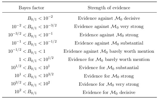
List of Bayes factors and their inference convention according to Jeffreys’ scale [5].
Markov Chain Monte Carlo
The goal of a Bayesian inference is to maintain the full posterior probability distribution. The models in question may contain a large number of parameters and so such a large dimensionality makes analytical evaluations and integrations of the posterior distribution unfeasible. Instead the posterior distribution can be approximated using Markov Chain Monte Carlo (MCMC) sampling algorithms. As the name suggests these are based on Markov chains which describe a sequence of random variables \(\Theta_0,\Theta_1,\dots\) that can be thought of as evolving over time, with probability of transition depending on the immediate past variable, \(P\left(\Theta_{k+1}\in A\middle|\theta_0,\theta_1,\dots,\theta_k\right)= P\left(\Theta_{k+1}\in A\middle|\theta_k\right)\) [6]. In an MCMC algorithm, Markov chains are generated by a simulation of walkers which randomly walk the parameter space according to an algorithm such that the distribution of the chains asymptotically reaches a target density \(f\left(\theta\right)\) that is unique and stationary (i.e. no longer evolving). This technique is particularly useful as the chains generated for the posterior distribution can automatically provide the chains of any marginalised distribution, e.g. a marginalisation over any or all of the nuisance parameters.
The Metropolis-Hastings (MH) algorithm [7] is the most well known MCMC algorithm and is shown in this algorithm:
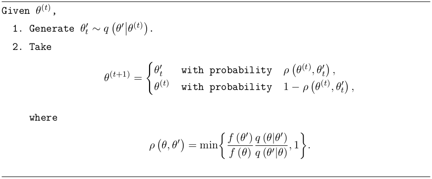
An initialisation state (seed) is first chosen, \(\theta^{(t)}\). The distribution \(q\left(\theta'\middle|\theta\right)\), called the proposal distribution, is drawn from in order to propose a candidate state \(\theta'_t\) to transition to. Commonly a Gaussian distribution is used here. Then the MH acceptance probability, \(\rho\left(\theta,\theta'\right)\) defines the probability of either accepting the candidate state \(\theta'_t\), or repeating the state \(\theta^{(t)}\) for the next step in the Markov chain. The acceptance probability always accepts the state \(\theta'_t\) such that the ratio \(f\left(\theta'_t\right)/\,q\left(\theta'_t\middle| \theta^{(t)}\right)\) has increased compared with the previous state \(f\left(\theta^{(t)}\right)/\,q\left(\theta^{(t)}\middle|\theta'_t\right)\), where \(f\) is the target density. Importantly, in the case that the target density is the posterior distribution, \(f\left(\theta\right)=\pi\left(\theta\middle|\textbf{x}\right)\), the acceptance probability only depends on the ratio of posteriors \(\pi\left(\theta'\middle|\textbf{x}\right)/\pi\left(\theta\middle|\textbf{x}\right)\), crucially cancelling out the difficult to calculate marginal distribution \(m\left(\textbf{x}\right)\). As the chain evolves, the target density relaxes to a stationary state of samples which, in our case, can be used to map out the posterior distribution.
To reduce the impact of any biases arising from the choice of the initialisation state, typically the first few chains after a burn-in period are discarded, after which the chains should approximate better the target density \(f\). While the MH algorithm forms the foundation of all MCMC algorithms, its direct application has two disadvantages. First the proposal distribution \(q\left(\theta'\middle|\theta\right)\) must be chosen carefully and secondly the chains can get caught in local modes of the target density. More bespoke and sophisticated implementations of the MH algorithm exist, such as affine invariant algorithms [8] which use already-drawn samples to define the proposal distribution or nested sampling algorithms [9], designed to compute the evidence \(\mathcal{Z}\). Both these types will be used in the Bayesian approach of this analysis. A more in depth look into the topic of MCMC algorithms is discussed in detail in Robert and Casella [6] or Collin [10].
Anarchic Sampling
As with any Bayesian based inference, the prior distribution used for a given parameter needs to be chosen carefully. In this analysis, a further technology needs to be introduced in order to ensure the prior distribution is not biasing any drawn inferences. More specifically, the priors on the standard model mixing parameters are of concern. These parameters are defined in the Physics section as a representation of the \(3\times3\) unitary mixing matrix \(U\), in such a way that any valid combination of the mixing angles can be mapped into a unitary matrix. The ideal and most ignorant choice of prior here is one in which there is no distinction among the three neutrino flavors, compatible with the hypothesis of neutrino mixing anarchy, which is the hypothesis that \(U\) can be described as a result of random draws from an unbiased distribution of unitary \(3\times3\) matrices [11], [12], [13], [14]. Simply using a flat prior on the mixing angles however, does not mean that the prior on the elements of \(U\) is also flat. Indeed doing this would introduce a significant bias for the elements of \(U\). Statistical techniques used in the study of neutrino mixing anarchy will be borrowed in order to ensure that \(U\) is sampled in an unbiased way. Here, the anarchy hypothesis requires the probability measure of the neutrino mixing matrix to be invariant under changes of basis for the three generations. This is the central assumption of basis independence and from this, distributions over the mixing angles are determined by the integration invariant Haar measure [13]. For the group \(U(3)\) the Haar measure is given by the volume element \(\text{d} U\), which can be written using the mixing angles parameterization:
which says that the Haar measure for the group \(U(3)\) is flat in \(\sin^2\theta_{12}\), \(\cos^4\theta_{13}\), \(\sin^2\theta_{23}\) and \(\delta\). Therefore, in order to ensure the distribution over the mixing matrix \(U\) is unbiased, the prior on the mixing angles must be chosen according to this Haar measure, i.e. in \(\sin^2\theta_{12}\), \(\cos^4\theta_{13}\), \(\sin^2\theta_{23}\) and \(\delta\). You can see an example on this in action in the Examples notebooks.
This also needs to be considered in the case of a flavor composition measurement using sampling techniques in a Bayesian approach. In this case, the posterior of the measured composition \(f_{\alpha,\oplus}\) is sampled over as the parameters of interest. Here, the effective number of parameters can be reduced from three to two due to the requirement \(\sum_\alpha f_{\alpha,\oplus}=1\). Therefore, the prior on these two parameters must be determined by Haar measure of the flavor composition volume element, \(\text{d} f_{e,\oplus}\wedge\text{d} f_{\mu,\oplus}\wedge\text{d} f_{\tau,\oplus}\). The following flavor angles parameterization is found to be sufficient:
| [1] | Casella, G. & Berger, R. Statistical Inference isbn: 9780534243128. https://books.google.co.uk/books?id=0x_vAAAAMAAJ (Thomson Learning, 2002). |
| [2] | Neyman, J. & Pearson, E. S. On the Problem of the Most Efficient Tests of Statistical Hypotheses. Phil. Trans. Roy. Soc. Lond. A231, 289–337 (1933). |
| [3] | Wilks, S. S. The Large-Sample Distribution of the Likelihood Ratio for Testing Composite Hypotheses. Annals Math. Statist. 9, 60–62 (1938). |
| [4] | Bayes, R. An essay toward solving a problem in the doctrine of chances. Phil. Trans. Roy. Soc. Lond. 53, 370–418 (1764). |
| [5] | (1, 2) Jeffreys, H. The Theory of Probability isbn: 9780198503682, 9780198531937, 0198531931. https://global.oup.com/academic/product/the-theory-of-probability-9780198503682?cc=au&lang=en&#(1939). |
| [6] | (1, 2, 3) Robert, C. & Casella, G. Monte Carlo Statistical Methods isbn: 9781475730715. https://books.google.co.uk/books?id=lrvfBwAAQBAJ (Springer New York, 2013) |
| [7] | (1, 2) Hastings, W. K. Monte Carlo sampling methods using Markov chains and their applications. Biometrika 57, 97–109. issn: 0006-3444 (Apr. 1970). |
| [8] | Goodman, J. & Weare, J. Ensemble samplers with affine invariance. Communications in Applied Mathematics and Computational Science, Vol. 5, No. 1, p. 65-80, 2010 5, 65–80 (2010). |
| [9] | Skilling, J. Nested Sampling. AIP Conference Proceedings 735, 395–405 (2004) |
| [10] | Collin, G. L. Neutrinos, neurons and neutron stars : applications of new statistical and analysis techniques to particle and astrophysics PhD thesis (Massachusetts Institute of Technology, 2018). http://hdl.handle.net/1721.1/118817. |
| [11] | De Gouvea, A. & Murayama, H. Neutrino Mixing Anarchy: Alive and Kicking. Phys. Lett. B747, 479–483 (2015). |
| [12] | Hall, L. J., Murayama, H. & Weiner, N. Neutrino mass anarchy. Phys. Rev. Lett. 84, 2572–2575 (2000). |
| [13] | (1, 2) Haba, N. & Murayama, H. Anarchy and hierarchy. Phys. Rev. D63, 053010 (2001). |
| [14] | De Gouvea, A. & Murayama, H. Statistical test of anarchy. Phys. Lett. B573, 94–100 (2003). |