Physics
Neutrinos
Introduction
The name neutrino was coined to describe a then hypothetical particle suggested by Wolfgang Pauli in the 1930’s [1]. Pauli’s idea was that of a neutral, weakly interacting particle having a very small mass. He proposed this particle could be used to explain the spectrum of electrons emitted by \(\beta\)-decays of atomic nuclei, which was of considerable controversy at the time. The observed spectrum of these electrons is continuous [2], which is incompatible with the two-body decay description successfully used to describe discrete spectral lines in \(\alpha\)- and \(\gamma\)- decay of atomic nuclei. As Pauli observed, by describing \(\beta\)-decay as a three-body decay instead, releasing both an electron and his proposed particle, one can explain the continuous \(\beta\)-decay spectrum. Soon after discovery of the neutron [3], Enrico Fermi used Pauli’s light neutral particle as an essential ingredient in his successful theory of \(\beta\)-decay, giving the neutrino it’s name as a play on words of little neutron in Italian [4].
It was not until some 20 years later that the discovery of the neutrino was realised. It was eventually understood that neutrinos came in three distinct flavors \(\left (\nu_e,\nu_\mu,\nu_\tau\right )\) along with their associated antiparticles \(\left (\bar{\nu}_e,\bar{\nu}_\mu,\bar{\nu}_\tau\right)\).
Neutrino Mixing
For the three massive neutrinos, the flavor eigenstates of the neutrino \(\mid{\nu_\alpha}>\), \(\alpha\in\{e,\mu,\tau\}\), are related to the mass eigenstates \(\mid{\nu_i}>\), \(i\in\{1,2,3\}\) via a unitary mixing matrix \(U_{\alpha i}\) known as the PMNS matrix [5], [6]:
This relationship can be seen better in this image:
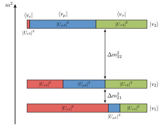
Graphical representation of the relationship between the neutrino flavor and mass eigenstates. The three mass eigenstates are depicted as three boxes, coloured such that the relative area gives the probability of finding the corresponding flavor neutrino in that given mass state.
The time evolution of the flavor eigenstate as the neutrino propagates is given by:
The oscillation probability gives the probability that a neutrino produced in a flavor state \(\alpha\) is then detected in a flavor state \(\beta\) after a propagation distance \(L\):
where the relation \(<{\nu_i}|{\nu_j}>=\delta_{ij}\) was used. Expanding this expression gives [7]:
where \(\Delta m_{ij}^2=m_i^2-m_j^2\). Note that for neutrino oscillations to occur, there must be at least one non-zero \(\Delta m_{ij}^2\) and therefore there must exist at least one non-zero neutrino mass state.
The mixing matrix can be parameterized using the standard factorization [8]:
where \(s_{ij}\equiv\sin\theta_{ij}\), \(c_{ij}\equiv\cos\theta_{ij}\), \(\theta_{ij}\) are the three mixing angles and \(\delta\) is the CP violating phase. Overall phases in the mixing matrix do not affect neutrino oscillations, which only depend on quartic products, and so they have been omitted. Therefore, this gives a total of six independent free parameters describing neutrino oscillations for three neutrino flavors in a vacuum. This table outlines the current knowledge of these parameters determined by a fit to global data [9]:
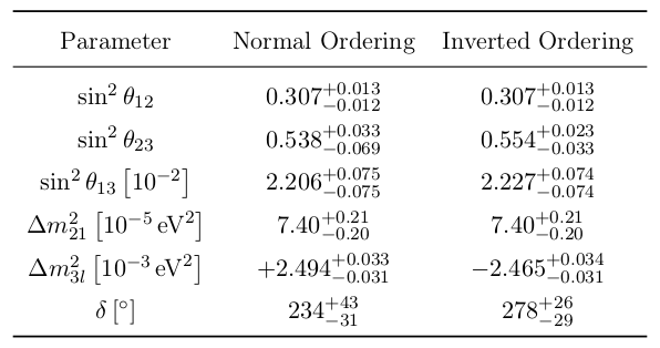
Three neutrino flavor oscillation parameters from a fit to global data [9].
This table shows two columns of values, normal ordering and inverted ordering corresponding to the case where the mass of \(\nu_3\) is greater than the mass of \(\nu_1\) or the mass of \(\nu_1\) is greater than the mass of \(\nu_3\), respectively. The experimental determination of this mass ordering is ongoing.
Astrophysical Neutrinos
The origin and acceleration mechanism of ultra-high-energy cosmic rays is still unknown. The difficulty comes from the fact that the cosmic rays are bent by interstellar magnetic fields, and so their arrival direction on Earth does not point back to their sources. The observation of these ultra-high-energy cosmic rays supports the existence of neutrino production at the sources of a similar energy range - an astrophysical neutrino flux. Neutrinos are electrically neutral, so are not perturbed by interstellar magnetic fields, and they also have a small enough interaction cross-section to escape from dense regions. This makes them ideal messengers to help identify the sources of cosmic rays:
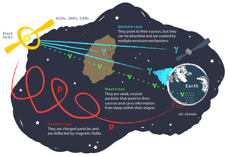
Neutrinos as messengers of astrophysical objects. Exotic astrophysical objects produce high-energy cosmic rays, photons and neutrinos, which can be detected on Earth. Credit: IceCube, NSF.
Ultra-high-energy cosmic rays detected on Earth manifestly succeed in escaping their sources, therefore these sources must be optically thin compared to the Earth’s atmosphere. Thus, the following interactions of the accelerated protons are expected to be more important than lengthy shower processes. High-energy protons can interact with photons as such:
They can also interact with other hadrons:
Importantly, final states here tend to produce pions which decay into either photons if neutral, \(\pi^0\rightarrow\gamma\gamma\), or if they are charged they decay into charged leptons and neutrinos. The neutral and charged pions are produced in similar amounts, meaning that the neutrino and photon fluxes are related. Indeed, the diffuse astrophysical neutrino flux can be estimated through \(\gamma\)-ray astronomy [10].
Point source searches of neutrinos are also being pursued. In 2017, a multi-messenger approach which searched for \(\gamma\)-ray observations in coincidence with neutrinos coming from a particular source has successfully been able to identify for the very first time, a source of high-energy astrophysical neutrinos [11], [12].
Of particular interest is the composition of flavors produced at the source. In the simple pion decay model described above, the neutrino flavor composition (sometimes referred to as the neutrino flavor ratio) produced at the source is:
For all discussions on the astrophysical neutrino flavor composition, the neutrino and antineutrino fluxes will been summed over as it is not yet experimentally possible to distinguish between the two. In the case that the muon interacts in the source before it has a chance to decay, e.g.@ losing energy rapidly in strong magnetic fields or being absorbed in matter, only the \(\nu_\mu\) from the initial pion decay escapes and so the source flavor composition is simply:
Another popular model is one in which the produced flux is dominated by neutron decay, \(n\rightarrow p+e^-+\bar{\nu}_e\), which gives rise to a purely \(\nu_e\) component:
Production of \(\nu_\tau\) at the source is not expected in standard astrophysics models. However, even in the standard construction, the composition could vary between any of the three idealised models above, which can be represented as a source flavor composition of \((x:1-x:0)\), where \(x\) is the fraction of \(\nu_e\) and can vary between \(0\rightarrow1\).
Once the neutrinos escape the source, they are free to propagate in the vacuum. As discussed above, neutrinos can transform from one flavor to another. Astrophysical neutrinos have \(\mathcal{O}(\text{Mpc})\) or higher baselines, large enough that the mass eigenstates completely decouple. The astrophysical neutrinos detected on Earth are decoherent and are propagating in pure mass eigenstates. Taking this assumption greatly simplifies the transition probability as all the interference terms between the three mass eigenstates can be dropped, and all that is left is to convert from the propagating mass state to the flavor states:
where \(\phi_\alpha\) is the flux for a neutrino flavor \(\nu_\alpha\) and \(\phi_i\) is the flux for a neutrino mass state \(\nu_i\). The subscript \(\text{S}\) denotes the source and \(\oplus\) denotes as measured on Earth. The same result can be obtained in the plane wave picture of the neutrino mixing equations above and taking the limit \(L\rightarrow\infty\), thus this type of decoherent mixing is also known as oscillation-averaged neutrino mixing. From this, the flavor composition on Earth is defined as \(f_{\alpha,\oplus}=\phi_{\alpha,\oplus}/\sum_\alpha\phi_{\alpha,\oplus}\) and this can be calculated using the mixing matrix parameters the table above. For the three source models discussed above:
This can be visualised in a ternary plot, which you can make yourself by checking out the Examples section! The axes here are the fraction of each neutrino flavor as shown below. The coloured circle, square and triangle show the source flavor compositions. The arrows show the effect of neutrino mixing on the flavor composition. The unfilled circle, square and triangle show the corresponding measured flavor composition. Neutrino mixing during propagation has the effect of averaging out the flavor contributions, which is why the arrows point towards the centre of the triangle. This effect is more pronounced for \(\nu_\mu\leftrightarrow\nu_\tau\) due to the their larger mixings. Also shown on this figure in the hatched Standard Model area, is the region of measured flavor compositions containing all source models of \(\left(x:1-x:0\right)\), using Gaussian priors on the standard mixing angles. Therefore, this hatched area is the region in which all standard astrophysical models live.
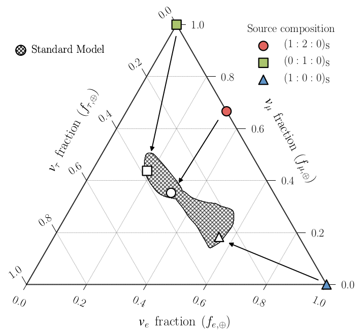
Astrophysical neutrino flavor composition ternary plot. Axes show the fraction of each neutrino flavor. Coloured shapes show 3 models for the source flavor composition. The arrows indicate the effect of neutrino mixing during propagation and the unfilled shapes show the corresponding measured flavor compositions. The hatched area shows the region in measured flavor space in which all standard astrophysical models live.
IceCube
Introduction
The IceCube Neutrino Obervatory is a cubic kilometre photomultiplier array embedded in the extremely thick and clear glacial ice located near the geographic South Pole in Antarctica. The IceCube array is made up of 5160 purpose built Digital Optical Modules (DOMs) which are deployed on 86 cables between 1450 and 2450 m below the ground. The interaction of a neutrino releases a burst of light in the detector, which is detected by this array of DOMs. The timing and intensity of these photons form the raw data set at IceCube. This data is analysed so that we can learn more about the properties of neutrinos. You can checkout some cool animations of how an event looks like in IceCube on this website.
A schematic layout of IceCube is shown below. The IceCube In-Ice array is made up of 5160 purpose built Digital Optical Modules (DOMs) which are deployed on 86 strings (or cables) between 1450 and 2450 m below the ground. The inner string separation is 125 m with a vertical DOM separation of 17 m. Eight of the centrally located strings make up the subarray DeepCore which are sensitive to lower energy neutrinos. It achieves this through denser instrumentation, having an inner string separation of 60 m and a vertical DOM separation of 7 m. A surface air shower array, IceTop, is instrumented on the surface and consists of a set of frozen water tanks which act as a veto against the background cosmic rays.
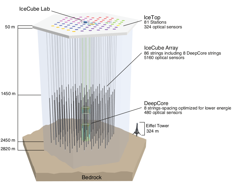
The IceCube neutrino observatory with the In-Ice array, its subarray DeepCore and the cosmic ray shower array IceTop.
Event Signatures
Cherenkov telescope arrays such as IceCube are able to classify the properties of a neutrino event by looking at the morphology of photon hits across its PMT array. There are two main types of neutrino event signatures at IceCube - tracks and cascades.
Tracks are predominantly made by muons which are directly produced by neutrinos in the charged current \(\nu_\mu\) interaction channel. Muons have a long lifetime, \(\sim\) 2 \(\mu\) s at rest, and in ice they have relatively low energy losses. Therefore, as shown in in the figure below, a high-energy muon travelling through the IceCube array will leave a long trail of hits. These features, along with the timing information of hits across the DOMs, help in determining the directionality of the muon, giving an angular resolution typically around \(0.5-1^\circ\) [13]. At energies of concern here, there is little deviation between the direction of the neutrino and the induced muon as they are both heavily boosted. Therefore, this pointing ability of tracks makes them the most attractive events to use for point source searches. Energy reconstruction is more complicated, however. At the lower energies (\(\lesssim100\) GeV), the muon’s range is short enough that it is able to deposit all its energy inside the detector. This is the ideal situation for a good energy reconstruction as the IceCube array acts as a calorimeter, so the total deposited charge is proportional to the energy of the muon. At higher energies, the range of the muon is typically greater than the length of the detector. Therefore the energy of muon must be extrapolated from the portion of energy deposited inside the detector. This is particularly challenging for muons which are not produced inside the detector, for which only a lower bound can be made. The typical approach taken to reconstruct the muon is to segment the reconstruction along the track. In this way, biases from stochastic variations of the energy loss can be minimised by applying some averaging over each segment. In each segment, the mean \(\text{d} E/\text{d} x\) is determined, which is then roughly proportional to the muon momentum. The energy resolution improves with the muon energy up to an uncertainty of a factor of 2 [14]. For more details on this see the IceCube energy reconstruction methods publication [15].
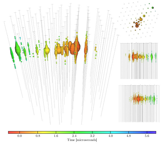
A track event initiated by a CC muon neutrino interaction in the detector. The muon deposits 74 TeV before escaping.
Cascades are created as a result of hadronic cascades and/or EM cascades. Neutral current interactions and CC \(\nu_e\) interactions are the channels in which a pure cascade is created, and an example of one is shown in the figure below. However, this does not mean that neutrino events produce exclusively one type of signature, in fact all high-energy neutrino-nucleon events produce at least a hadronic cascade at the interaction vertex. Characteristic of a cascade is the isotropic deposition of energy in a localised region near the neutrino vertex. Contrary to tracks, cascade events have much shorter typical lengths and so the entire energy deposition is easily contained within the detector array. This is ideal for energy reconstruction giving a deposited energy resolution of \(\sim\) 15% at neutrino energies above 10 TeV [15]. Inferring the true neutrino energy is more difficult, however, as IceCube is not capable of resolving the difference between EM showers and hadronic showers, which potentially have a large amount of missing energy, leading to \(\sim\) 15% lower light yield compared to an equivalent EM shower. Deposited energy is reconstructed using an EM shower hypothesis, and therefore this quantity gives the lower limit of the neutrino energy. Directional reconstruction is more challenging than for tracks and is done by looking for timing/light intensity anisotropies around the interaction vertex. The deviations are small, but it is expected that the light deposition in the forward direction is greater. Typical angular resolutions are \(10-15^\circ\) [16].
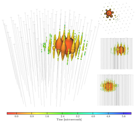
A cascade event initiated by a neutrino interaction in the detector. The cascade deposits 1070 TeV in the detector.
Not mentioned so far are the charged current \(\nu_\tau\) interactions, which for energies \(\gtrsim\) 1 PeV, can produce \(\tau\) which travels a detectable distance before decaying. This provides a unique signature for such events. The initial \(\nu_\tau\) interaction produces a hadronic cascade, followed by a track by the \(\tau\) itself, in turn followed by either a track from the \(\tau\)’s muonic decay (\(\tau^-\rightarrow\mu^-\bar{\nu}_\mu\nu_\tau\) with branching ratio \(\sim\) 17%), or a cascade from its other decays. Because of their distinctive signatures, such events are called double bangs or double cascades. See [17], [18] for more details.
| [1] | Pauli, W. Letter to Tübingen conference participants Web document. 1930. |
| [2] | Chadwick, J. Intensitätsverteilung im magnetischen Spectrum der \(\beta\)-Strahlen von radium B + C. Verhandl. Dtsc. Phys. Ges. 16, 383 (1914). |
| [3] | Chadwick, J. Possible Existence of a Neutron. Nature 129, 312 (1932). |
| [4] | Fermi, E. An attempt of a theory of beta radiation. 1. Z. Phys. 88, 161–177 (1934). |
| [5] | Pontecorvo, B. Neutrino Experiments and the Problem of Conservation of Leptonic Charge. Sov. Phys. JETP 26. [Zh. Eksp. Teor. Fiz.53,1717(1967)], 984–988 (1968). |
| [6] | Maki, Z., Nakagawa, M. & Sakata, S. Remarks on the unified model of elementary particles. Prog. Theor. Phys. 28. [,34(1962)], 870–880 (1962). |
| [7] | Giunti, C. & Kim, C. W. Fundamentals of Neutrino Physics and Astrophysics isbn: 9780198508717 (2007). |
| [8] | Beringer, J. et al. Review of Particle Physics (RPP). Phys. Rev. D86, 010001 (2012). |
| [9] | (1, 2) Esteban, I., Gonzalez-Garcia, M. C., Maltoni, M., Martinez-Soler, I. & Schwetz, T. Updated fit to three neutrino mixing: exploring the accelerator-reactor complemen- tarity. JHEP 01, 087 (2017). |
| [10] | Kappes, A., Hinton, J., Stegmann, C. & Aharonian, F. A. Potential Neutrino Signals from Galactic Gamma-Ray Sources. Astrophys. J. 656. [Erratum: Astrophys. J.661,1348(2007)], 870–896 (2007). |
| [11] | Aartsen, M. G. et al. Multimessenger observations of a flaring blazar coincident with high-energy neutrino IceCube-170922A. Science 361, eaat1378 (2018). |
| [12] | Aartsen, M. G. et al. Neutrino emission from the direction of the blazar TXS 0506+056 prior to the IceCube-170922A alert. Science 361, 147–151 (2018). |
| [13] | Aartsen, M. G. et al. All-sky Search for Time-integrated Neutrino Emission from Astrophysical Sources with 7 yr of IceCube Data. Astrophys. J. 835, 151 (2017). |
| [14] | Weaver, C. Evidence for Astrophysical Muon Neutrinos from the Northern Sky PhD thesis (Wisconsin U., Madison, 2015). https://docushare.icecube.wisc.edu/dsweb/Get/Document-73829/. |
| [15] | (1, 2) Aartsen, M. G. et al. Energy Reconstruction Methods in the IceCube Neutrino Telescope. JINST 9, P03009 (2014). |
| [16] | Aartsen, M. G. et al. Evidence for High-Energy Extraterrestrial Neutrinos at the IceCube Detector. Science 342, 1242856 (2013). |
| [17] | Hallen, P. On the Measurement of High-Energy Tau Neutrinos with IceCube PhD thesis (RWTH Aachen University, 2013). https://www.institut3b.physik.rwth-aachen.de/global/show_document.asp?id=aaaaaaaaaapwhzq. |
| [18] | Xu, D. L. Search for astrophysical tau neutrinos in three years of IceCube data PhD thesis (The University of Alabama, 2015). http://acumen.lib.ua.edu/content/u0015/0000001/0001906/u0015_0000001_0001906.pdf |